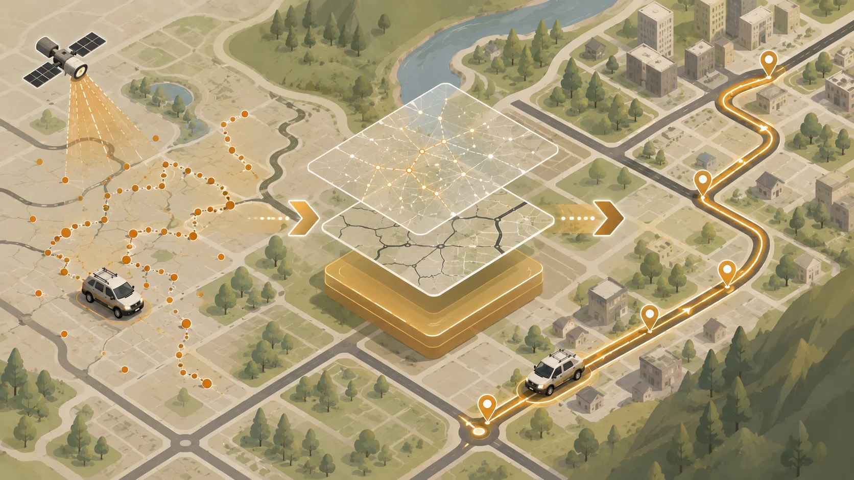
Map matching is the process of taking a sequence of raw, noisy GPS coordinates and aligning them to the actual roads a vehicle or device was really on. It’s a small correction step with a large downstream effect, since almost nothing built on top of GPS data works well until this problem is solved.
The core issue is simple: GPS is never perfectly accurate. A phone in a moving car regularly reports positions 5 to 20 meters off the real road, and without correction, those raw points can appear to sit inside a building, in the middle of a river, or in a parking lot next to the street the vehicle actually drove down. Plot 500 raw GPS points from an hour-long drive on a map with no correction applied, and the result looks less like a route and more like a scatter of dots loosely following the shape of a road, readable to a human squinting at it, useless to any system trying to calculate mileage, road type, or arrival time from it directly.
This guide covers what map matching actually does, how the algorithm behind it works, what a real API request and response look like, where it breaks in practice, and how to add it to a GPS tracking application. Farun’s Map Match endpoint is used as the working example throughout, alongside honest comparisons to how other providers handle the same problem, since the underlying algorithmic ideas are shared across almost every serious implementation in this space rather than being unique proprietary secrets.
What Is Map Matching?
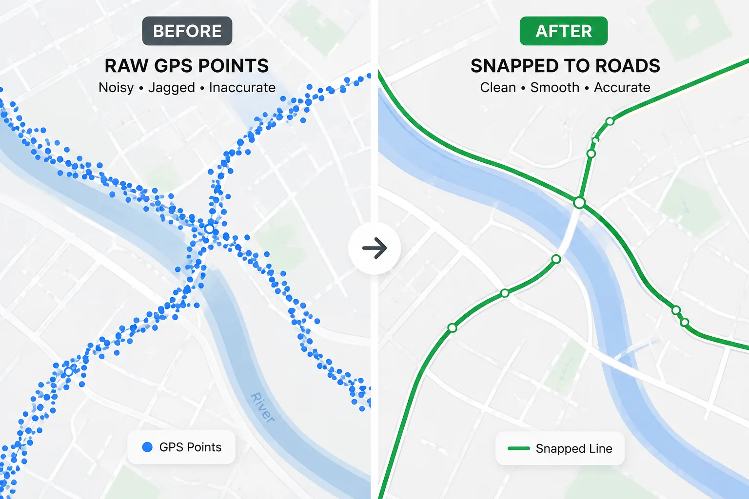
Map matching is the process of aligning a sequence of GPS coordinates to the road network they most likely represent, correcting for GPS error so that a “trace”, a path of raw points becomes a clean route that actually follows real streets.
Map matching is different from routing in a specific, important way: routing calculates a path before a trip happens, while map matching reconstructs the most likely path after GPS points have already been recorded, or as they stream in during a trip already in progress. The practical outcome is straightforward, a jagged, zig-zagging line of raw GPS dots becomes a smooth line that follows actual road geometry. “Snap to roads” and “map matching” are used interchangeably in most product documentation, though map matching is the more precise and widely used academic term, as Wikipedia’s page on map matching lays out in more formal terms.
What Is a GPS Trace?
A GPS trace is a time-ordered sequence of latitude/longitude coordinates recorded by a device as it moves, usually with a timestamp and sometimes speed or heading attached to each point.
The raw shape of trace data is simple: an array of points, each with lat, lng, and a timestamp, the input format nearly every map matching API expects, including Farun’s Map Match endpoint. Sampling rate, how often a point is recorded, every second, every 5 seconds, or every 30 seconds is the single biggest factor in how usable a trace is before it even reaches a matching algorithm. Common trace sources include phone GPS, dedicated GNSS hardware like GPS Navigator, vehicle telematics units, and fitness or cycling computers.
Why Do GPS Traces Need to Be Snapped to Roads?
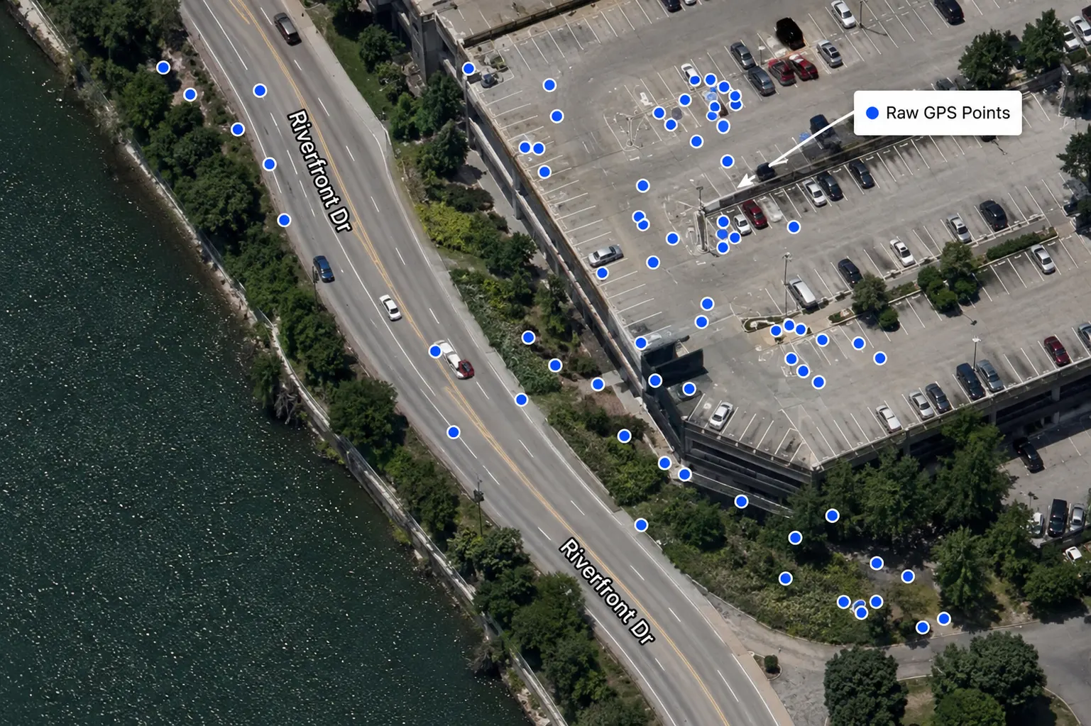
Raw GPS traces need to be snapped to roads because consumer GPS receivers are accurate to roughly 5–15 meters under open sky, and far worse near tall buildings, tunnels, or dense tree cover, error that routinely places recorded points off the actual road entirely.
The physical causes are straightforward: signal multipath off buildings, atmospheric interference, and receiver quality all shift a reported position away from the true one. The downstream consequences are concrete and costly, wrong-looking driver history maps, inflated mileage calculations, and incorrect road-type attribution for anything built on top of that trace. This isn’t a rare edge case. It’s the default state of essentially all consumer, and even most commercial, GPS data before correction, which is exactly why routing engines and mapping platforms treat map matching as a core capability rather than an optional add-on.
What Is the Difference Between Map Matching and Simple Snap-to-Nearest-Road?
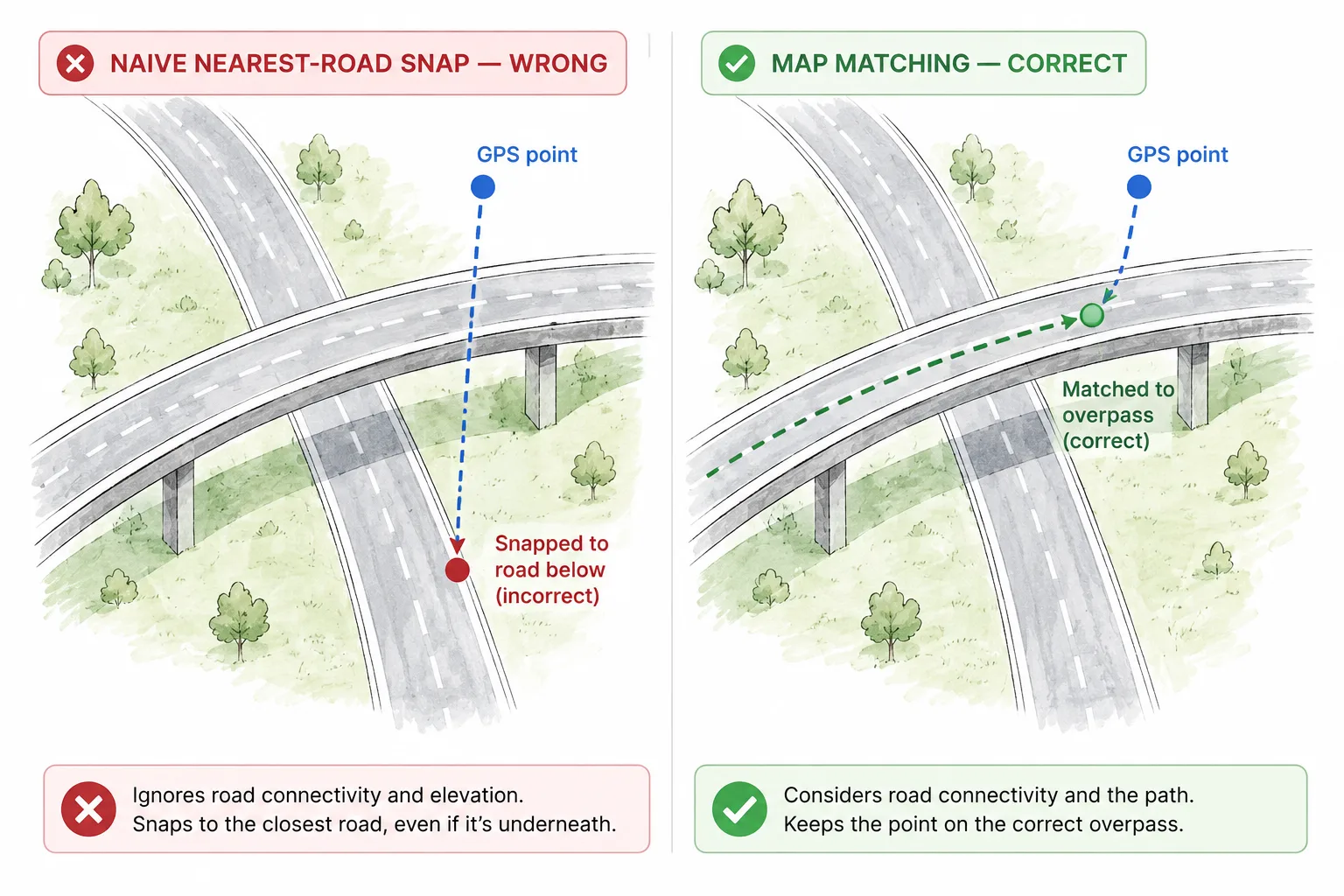
Snap-to-nearest-road moves each point individually to the closest road segment with no memory of previous points. Map matching considers the whole sequence together, using road connectivity and travel plausibility to pick the path that makes sense as a continuous route, not just the closest line to each dot.
A concrete failure case makes the difference obvious: a GPS point recorded on an overpass can get snapped to the road directly underneath it if only nearest-distance is considered, producing a physically impossible route. Map matching evaluates whether moving from one candidate road segment to the next candidate segment is actually possible to drive, given real road connections, nearest-point snapping has no concept of this at all. This distinction is the entire reason map matching exists as its own discipline rather than being a one-line geometry function, and it’s the same distinction that separates a genuinely useful GPS trace cleanup tool from a cosmetic one.
How Does a Map Matching Algorithm Actually Work?
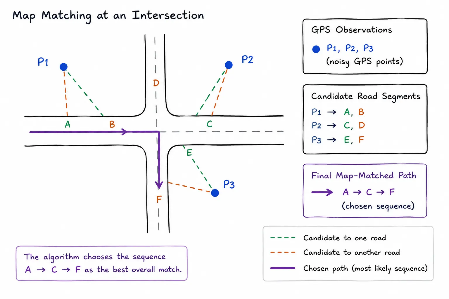
Most modern map matching uses a Hidden Markov Model (HMM), which treats each GPS point as a noisy clue about a hidden “true” road position, then finds the most likely sequence of road segments across the whole trace by balancing how close each candidate is to the GPS point against how plausible it is to travel between consecutive candidates.
The idea breaks into two plain-English pieces. First, emission probability, how likely is it that this GPS point came from being on this particular nearby road segment, based on distance. A GPS point sitting 3 meters from Road A and 40 meters from Road B makes Road A a far more probable emission source than Road B, all else being equal. Second, transition probability, how likely is it that the vehicle actually traveled from the previous candidate segment to this candidate segment, based on real road-network distance versus straight-line distance, not just raw proximity.
Here’s a simplified version of how that plays out. Picture three consecutive GPS points recorded near a busy four-way intersection, each with two or three nearby candidate road segments. Point one sits closest to the eastbound lane of Main Street, but also has a weaker candidate on a side street a few meters further away. Point two, recorded a few seconds later, sits near the intersection itself, where several road segments converge. Point three sits clearly on the continuation of Main Street heading east. A naive nearest-point approach might snap point two to whichever segment happens to be geometrically closest, even if that segment doesn’t actually connect to where point one and point three ended up. The HMM approach instead asks a different question for the middle point: given where point one most likely was and where point three most likely was, which candidate at point two makes the whole three-point sequence physically drivable and reasonably close to the raw data at every step? That question, evaluated across the entire trace at once, not one point at a time is what separates map matching from simple snapping, and it’s the same core logic whether the trace has three points or three thousand.
The foundational version of this approach comes from a well-cited 2009 Microsoft Research paper by Paul Newson and John Krumm, Hidden Markov Map Matching Through Noise and Sparseness, and nearly every production map matching service in use today, including open-source engines like GraphHopper’s map-matching module, which explicitly credits this paper in its own source code and implements the same Viterbi algorithm to solve it efficiently, builds on some variation of it. That’s worth knowing on its own: the field isn’t a collection of unrelated proprietary tricks, it’s mostly one shared algorithmic idea implemented slightly differently by each provider, which is also why accuracy tends to converge across serious implementations once each one is properly tuned.
What Inputs Does a Map Matching API Need?
A map matching API needs an ordered list of latitude/longitude coordinates with timestamps, plus a travel profile such as driving, cycling, or walking, timestamps and profile both directly affect which candidate roads get considered plausible.
The core required fields are an ordered coordinate array, a timestamp per point (critical for transition-probability calculations), and a costing or profile parameter. Common optional fields include an accuracy radius per point, if the device reports its own GPS confidence, plus heading and speed, both of which sharpen candidate selection when available. One practical constraint worth flagging upfront: most map matching services, including Farun’s Map Match endpoint, cap how many points can be sent in a single request, so long traces from a multi-hour trip usually need to be chunked into smaller batches before submission.
What Does a Map Matching API Response Include?
A map matching API response typically includes the snapped route geometry, a confidence or match-quality score, and, depending on the service, either turn-by-turn-style route data or detailed attributes for each matched road segment, such as road class or speed limit.
The geometry output is a clean line, often as an encoded polyline or GeoJSON, following actual roads instead of the raw jagged input trace. Confidence scoring gives a signal for how well the input trace actually matched, which is useful for automatically flagging unreliable traces rather than trusting every result blindly. Some services split “matched geometry” and “matched attributes” into two genuinely separate response types, which is worth its own explanation, covered next.
What Is the Difference Between a Snapped Route and Matched Edge Attributes?
A snapped route returns the corrected path geometry, the line itself. Matched edge attributes return metadata about each road segment the trace passed through, such as road class, speed limit, or a road’s internal ID, the same input trace, but a very different kind of answer.
A concrete use-case split makes this clear: an app rendering “here’s where the driver actually went” on a map needs the snapped route, while an app calculating “how much of this trip was on a highway versus a residential street” needs the attribute output instead. Farun’s own Map Match endpoint is described specifically as returning “matched routes or edge attributes”, meaning both output shapes are available from the same underlying match depending on what the request asks for. This mirrors how Valhalla’s Map Matching service splits the same distinction between its trace_route and trace_attributes actions, a pattern that shows up across most mature map matching services once you look for it. A team building a driver-history feature and a team building a road-type risk model off the same GPS data may end up calling the same matching service twice, with different response expectations each time.
How Does GPS Sampling Rate Affect Map Matching Accuracy?
Higher sampling rates, more GPS points per minute, make map matching more accurate, since closely spaced points give the algorithm more evidence about which road was actually traveled. Points spaced 30 seconds or more apart start to introduce real ambiguity, especially near complex intersections.
Sampling every 1–5 seconds is considered high-frequency and produces reliable matches even in dense urban road networks. Sampling every 30–60 seconds is common in battery-conscious tracking apps and starts to produce genuine ambiguity about which of several nearby roads was used. The reason is straightforward: sparse points mean more distance between consecutive candidates, which means more possible road paths could plausibly connect them, giving the algorithm less evidence to rule out wrong answers. This is a real design trade-off every mobile app team faces, higher sampling rate improves match quality but drains battery and increases data usage faster, not a free choice either way.
What Causes Map Matching to Fail or Produce a Bad Match?
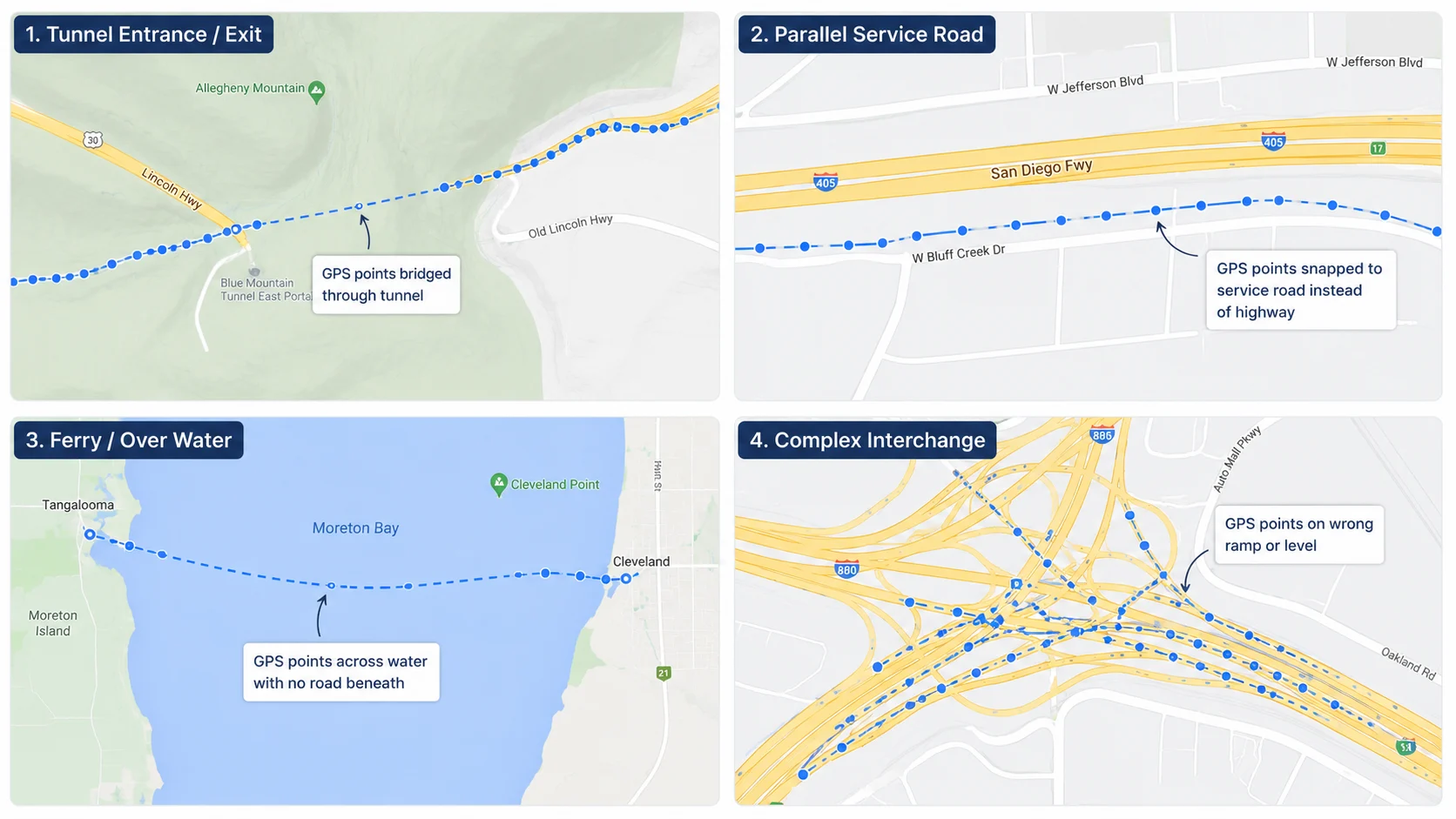
Map matching commonly fails in tunnels and parking structures where GPS is lost entirely, on parallel roads running close together such as service roads next to highways, and on ferries or private roads that aren’t in the underlying road network at all.
Tunnels and underground parking cause GPS signal to disappear completely, leaving a gap the algorithm has to bridge with a guess based on the points before and after, usually fine for a short tunnel, unreliable for a long one. Parallel roads, a service road running next to a highway, or two one-way streets running in opposite directions a few meters apart can genuinely confuse matching when GPS accuracy is worse than the distance between the two roads. Ferries and private roads cause a different kind of failure: if a route legitimately isn’t in the underlying road network, like a ferry crossing, a private driveway, or a construction detour, matching will force the trace onto the nearest road that does exist, producing a confidently wrong answer rather than an honest “no match.” Very low sampling rate combined with a complex intersection rounds out the list, two GPS points on either side of a busy interchange, recorded a minute apart, can match to several equally plausible routes through that interchange. These aren’t rare edge cases dreamed up for a blog post; they’re the specific, recurring scenarios that show up in almost every production GPS tracking system eventually, whether the traces come from road vehicles, marine vessels navigating coastal waters, or field equipment.
How Do You Handle Map Matching for Off-Road or Rural GPS Traces?
Off-road and rural traces need a wider search radius and a matching profile that includes unpaved tracks and minor roads, since default driving profiles tuned for cities often exclude the exact road types rural and agricultural GPS traces actually travel on.
The core problem: a matching service defaulting to a standard driving profile may not have unpaved farm tracks or forestry roads in its usable road graph at all, forcing points onto a distant paved road instead of the dirt track a vehicle actually used. Widening the candidate search radius specifically for rural use cases helps, since roads are sparser and the correct road may legitimately be farther from the raw GPS point than in a dense city grid. This matters directly for agricultural equipment tracking and rural fleet monitoring, the kind of workflow covered in more depth on Farun’s agriculture solutions, where elevation, rural routing, and terrain context already have to account for the same sparse-road reality that map matching does.
What Is the Difference Between Real-Time Map Matching and Batch Map Matching?
Real-time map matching processes a small, growing window of recent GPS points as a device moves, useful for live tracking. Batch map matching processes a complete, already-recorded trace all at once, producing a more accurate result since it has the full trip’s context available from the start.
The real-time constraint is straightforward: a live tracking app can only match against points that have already been received, so early-trip matches are naturally less certain than they’ll become once more of the route is known. Batch matching is more accurate specifically because having the entire trace available lets the algorithm use points after an ambiguous section to help resolve it, not just points before. The use-case split is clean: live driver-tracking dashboards need real-time matching, while trip-history analytics, mileage reporting, and insurance risk scoring are almost always batch use cases run after a trip completes.
How Does Map Matching Compare Across Providers?
Map matching providers differ mainly in underlying routing engine, point-count limits per request, output format, and whether both route geometry and road attributes are available from the same call.
| Provider | Engine basis | Point limit per request | Output types | Notes |
|---|---|---|---|---|
| Farun Map Match | OSRM-style road graph | See API docs | Matched route or edge attributes | Shares road-graph coverage with Farun’s Routing API |
OSRM /match | OSRM (self-hosted or hosted) | No hard API limit, practically batched | Matched route geometry | Free, open-source, self-hosted only |
Valhalla trace_route / trace_attributes | Valhalla | Large traces need chunking | Route or detailed attributes | Split endpoints for route vs. attributes, see the Valhalla docs |
| Mapbox Map Matching API | Mapbox Directions engine | 100 coordinates per request | Matched route | Hard 100-point cap, requires chunking, see Mapbox’s documentation |
| AWS Location SnapToRoads | Proprietary | Documented per-request limit | Snapped geometry + per-point confidence | Returns a confidence score per snapped point, per AWS’s own guide |
For most developers, the real differentiator isn’t raw accuracy, most HMM-based engines converge on similar quality once tuned, it’s operational details: point limits, self-hosting options, and whether attribute-level output is available without a second call. Anyone weighing a self-hosted option should also look at GraphHopper’s own map-matching module directly on GitHub, which documents its Viterbi-algorithm implementation of the same Newson-Krumm approach in enough detail to actually read the source.
The self-hosted-versus-hosted-API decision usually comes down to three questions, and it’s worth answering all three honestly before committing either way. First, how much operational overhead can the team actually absorb, self-hosting OSRM or GraphHopper means owning server infrastructure, road-graph updates, and uptime, not just an algorithm. Second, does the product need private infrastructure for data-residency or compliance reasons, in which case a hosted API’s terms of service may rule it out regardless of price. Third, what does request volume actually look like at scale, a hosted API’s per-request pricing is easy to reason about at low volume and can become the more expensive option only once volume gets large enough that self-hosting’s fixed infrastructure cost is clearly cheaper by comparison. Most teams starting out should default to a hosted API and revisit the self-hosted question only once volume or compliance actually forces it, rather than front-loading infrastructure work for a scale the product hasn’t reached yet.
Which Industries Rely on Map Matching the Most?
Fleet telematics, usage-based insurance, delivery analytics, ride-hailing, and transportation research are the heaviest users of map matching, each turning raw GPS traces into something road-aware and analyzable.
Fleet Telematics and Vehicle Tracking
Fleet management platforms depend on map matching to turn raw GPS pings from vehicles into clean, road-following trip histories drivers and managers can actually read. Farun’s fleet operations covers how this fits alongside routing, dispatch, and driver-facing tooling built on the same underlying road network.
Usage-Based Insurance and Risk Scoring
Insurers scoring driving behavior need to know not just where a vehicle was, but what kind of road it was on, highway driving and residential-street driving carry different risk profiles, and that distinction only exists after matching. Farun’s insurance solutions covers how road-type context feeds directly into underwriting and claims models.
Delivery and Logistics Analytics
Logistics teams use matched traces to verify actual driver routes against planned routes, measure real stop-to-stop travel time, and audit whether delivery routes match what was dispatched by the Optimized Route API in the first place. Farun’s logistics solutions covers the broader routing and dispatch context this data feeds into.
Ride-Hailing and Micromobility
Ride-hailing and scooter or bike-share platforms use map matching to reconstruct accurate trip paths for fare calculation, trip history, and safety review, especially in dense downtown cores with tall buildings, exactly the environment where raw GPS accuracy is at its worst and multipath error is most severe. A fare calculated from unmatched raw GPS distance in a dense downtown grid can overstate real trip distance noticeably once the zig-zag of raw point error is factored in, which is a direct revenue and customer-trust issue, not just a cosmetic mapping one.
Transportation Research and Traffic Studies
Academic and government transportation studies rely heavily on map matching to convert raw probe-vehicle GPS data into road-segment-level traffic flow and speed estimates, which is where a large share of published map matching research, including the foundational Newson-Krumm paper referenced earlier, originally came from. Without matching, a fleet of probe vehicles’ raw GPS traces can’t be reliably attributed to specific road segments at all, which makes segment-level average speed or congestion estimation effectively impossible at any real scale.
What File and Request Formats Does Map Matching Commonly Use?
Map matching requests are almost always sent as JSON containing an ordered coordinate array, while some open-source tools also accept GPX files directly as a more human-portable trace format.
Most APIs, including Farun’s Map Match endpoint, expect a plain JSON body: an array of coordinate objects, each carrying latitude, longitude, and a timestamp. GPX, an XML-based format originally built for GPS devices, is common in open-source tooling, GraphHopper’s map-matching web service accepts GPX files directly and can return matched results as GPX or JSON. Response formats lean toward GeoJSON or encoded polylines for geometry, and plain JSON arrays for attribute data, which keeps integration straightforward regardless of which provider a team ultimately picks.
What Are Common Mistakes When Using a Map Matching API?
The most common mistakes are sending points without timestamps, using the wrong travel profile, ignoring confidence scores, and trying to match extremely long traces in a single oversized request.
Sending coordinates without timestamps removes the information the algorithm needs to reason about plausible travel time between points, and matching quality drops noticeably as a result, especially at low sampling rates. Using a driving profile for a cycling or walking trace excludes footpaths and may apply one-way restrictions that don’t actually apply to a pedestrian, producing a route that’s technically road-following but practically wrong. Ignoring the confidence or match-quality score entirely treats a genuine warning signal as noise, a low-confidence match should be flagged, not silently trusted the same as a high-confidence one. Sending an entire multi-hour trace in one oversized request ignores that most services.
How Accurate Is Map Matching, and How Do You Measure It?
Map matching accuracy is typically measured as the percentage of matched road segments that agree with a known ground-truth route, and well-tuned HMM-based matchers on decent-quality traces commonly reach well above 90% segment-level agreement, though this drops significantly with sparse sampling or dense, ambiguous road networks.
There’s a practical way to test this without any special tooling: drive or walk a known route while logging GPS, run the resulting trace through a matching endpoint, then manually compare the matched output against the real path on a map. It’s a test almost any team could run in an afternoon before committing to a provider. Published academic accuracy figures, including the original Newson-Krumm evaluation, show accuracy degrading measurably as GPS sampling interval increases, accuracy isn’t a fixed number independent of input quality, it’s a function of it. One developer’s public write-up on Towards Data Science, “Map Matching done right using Valhalla’s Meili,” documents hitting exactly this issue in a real production project, including a rough error-rate estimate from a naive nearest-road approach before switching to proper HMM-based matching. It’s worth testing accuracy specifically in the geography a product will actually operate in.
A few concrete numbers help set expectations. The original Newson-Krumm evaluation found accuracy dropping from roughly 99% at a high sampling rate down into the 80s as the interval between GPS points stretched out, a reminder that “map matching accuracy” is really shorthand for “map matching accuracy at a specific sampling rate on a specific road network,” not a single fixed property of the algorithm itself. This is exactly why a five-minute self-test using a team’s own real devices, in the team’s own operating region, is worth more than trusting any single published accuracy figure at face value, including the numbers in this article.
FAQs About Map Matching APIs
Q1: Is map matching the same as routing?
A1: No. Routing calculates a path before a trip happens. Map matching reconstructs the most likely path a device already traveled, based on GPS points that were already recorded. Farun exposes both as separate endpoints, see Routing versus Map Match, since they solve opposite problems.
Q2: Does map matching need internet connectivity?
A2: Cloud-based map matching APIs need connectivity to send the trace and receive a result. Offline map matching is possible but requires the road network data and matching logic to be available locally on the device, as covered in the offline section above.
Q3: How many GPS points can I send in one map matching request?
A3: This varies significantly by provider, Mapbox caps requests around 100 coordinates, while others allow larger batches. Always check the specific provider’s documented limit.
Q4: What happens if my GPS trace has a big gap, like from a tunnel?
A4: Most map matching algorithms bridge short gaps using the points before and after, but very long gaps introduce real ambiguity about the exact path taken during the gap, as discussed in the failure-modes section above.
Q5: Can map matching correct GPS drift while a vehicle is parked?
A5: Not reliably. Map matching assumes movement along a road network, a stationary, drifting GPS signal in a parking lot doesn’t fit that assumption well and can produce erratic-looking matched output.
Q6: Do I need a separate map matching API, or does my routing API include it?
A6: Routing and map matching are usually separate endpoints, even from the same provider, since they solve opposite problems, routing looks forward, map matching looks backward at data that already exists.
Which Map Matching Approach Should You Use?
Use a cloud map matching API for most applications, self-hosted open-source engines like OSRM or GraphHopper for high-volume or privacy-sensitive workloads, and offline on-device matching only when connectivity genuinely can’t be guaranteed.
- Building a driver-history or trip-review feature → hosted map matching API, batch mode, like Farun’s Map Match endpoint.
- Live tracking dashboard → hosted API in real-time/streaming mode.
- Very high request volume or strict data-residency requirements → self-hosted OSRM or GraphHopper.
- Vehicles or vessels operating with unreliable connectivity → offline-capable hardware like GPS Navigator with bundled road data.